Pivot Table is one of the most powerful features of MS Excel which makes Excel one of the most sought after Data Analysis tool for every Data Analyst. Pivot Table can take very large data sets as input to summarise it all as required. While Pivot tables are extremely powerful, they can be very complicated too. But don't you worry as we are here to demystify Pivot Tables for you.

It may seem that Pivot tables are hard to master but it is actually way easier than you might have thought. Here we will be covering every bit about PIVOT tables which you must know in order to befriend PIVOT table and master the concept.

As briefly stated earlier, pivot table is a summary of your dataset which is in a form of a table to which you can assign various fields and data values in order to see data from multiple perspectives, enabling you to derive insights from your dataset. The more the rows and columns you have, more ways of arranging data you will have in order to compare the various forms and values which may help you get actionable insights which would have else remain hidden.

To reiterate, Pivot table gives you a way to group your data set in various ways or perspectives so that you are able to derive meaningful insights easily while making no changes to the original data.

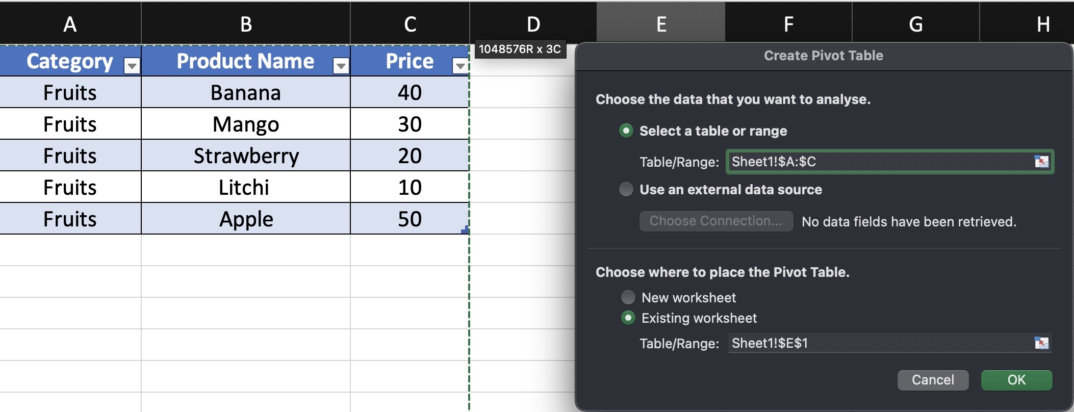
Pivot table may sound complex but it is really very easy. Imagine you have a table containing columns category = fruit, fruit name and prices. 

If you want to know the sum total of all category = fruit, either you can do sum of all rows of the table or you can create a pivot table where you will have category on the row side and prices towards the value side and you will get the desired data. You will be able to calculate average or any other operation as well.

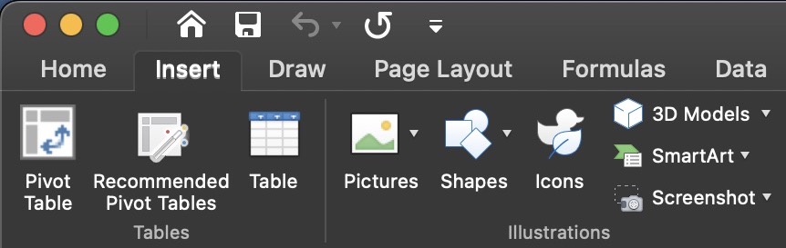
Once you have the data in your MS Excel worksheet, go to a new worksheet where you want to have the Pivot table. Move your cursor to the top menu and click on Insert Ribbon Menu, and choose the first option called Pivot Table.

Now when you will click on the Pivot Table option, you will get the Create Pivot Table screen. 

Two things have to be done here - You have to tell it where your data set is located and where you want to have your new Pivot Table.

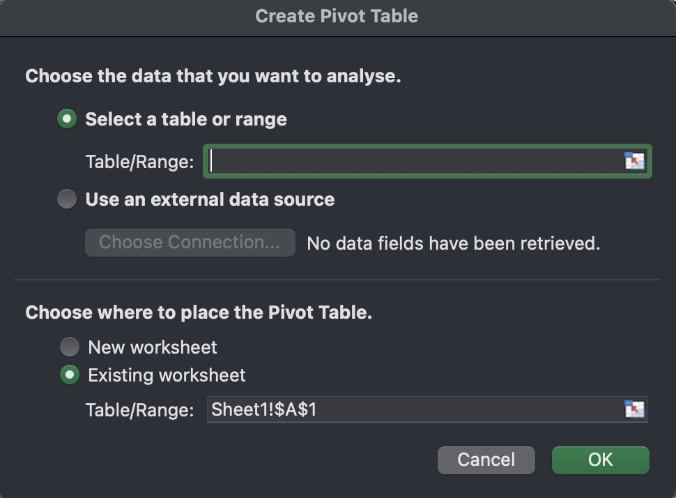
For entering the location where your data is location, click on the text box and then go to the worksheet where your data set is located. It is ideal to select entire columns so that you won't have to change the selection whereever there is any update in the data set. Once done, to choose where you want to place the Pivot Table, it must have the location already as you had earlier gone to a new worksheet and a cell was already selected. Click on OK to create a blank Pivot Table.

This is how a blank Pivot Table appears.